Simple use case

The tutrial introduces an usage of grasp2alm which is based on Planck LevelS beam function.

import grasp2alm as g2a
import numpy as np
import matplotlib.pyplot as plt
import healpy as hp

Let’s load beam files. GRASP grid and cut format are covered.

gridfile = "../../test/beam_files/test.grd"
cutfile = "../../test/beam_files/test.cut"
grid = g2a.BeamGrid(gridfile)
cut = g2a.BeamCut(cutfile)

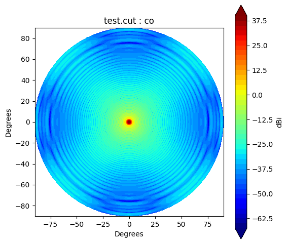
BeamGrid, BeamCut and BeamPolar class has a method to plot a beam. It has unit as dBi, and its operation as following:

\(\mathrm{dBi} = 10\log_{10}(I)\)

where \(I\) representes intensity of the beam.

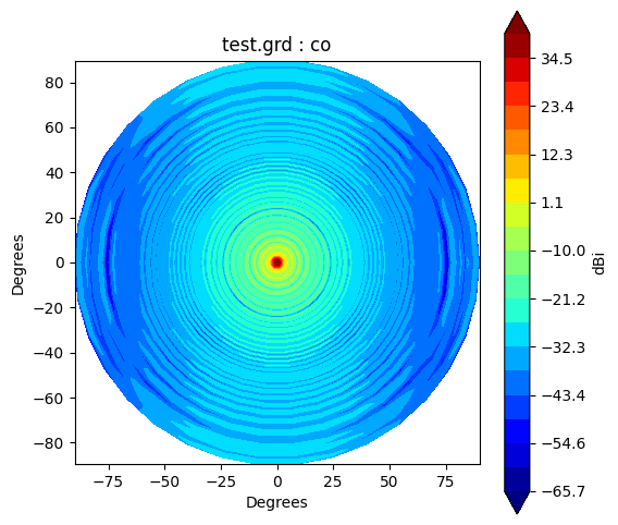
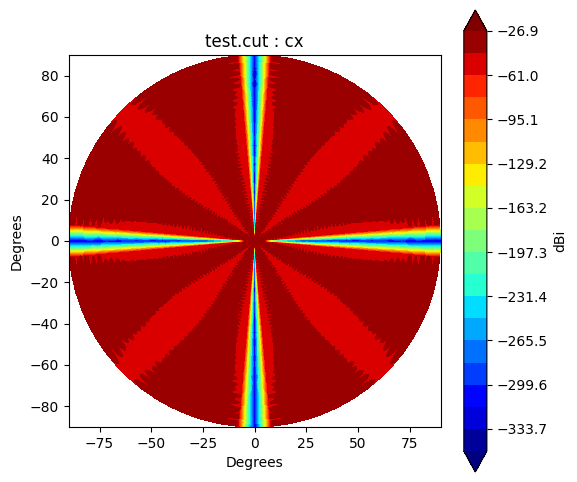
The co-pol (co) beam and cross-pol (cx) beam can be controled by argument pol.

grid.plot(pol='co')
cut.plot(pol='cx')

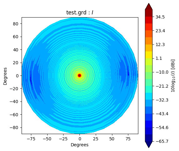
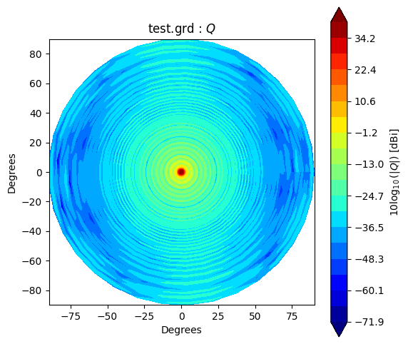
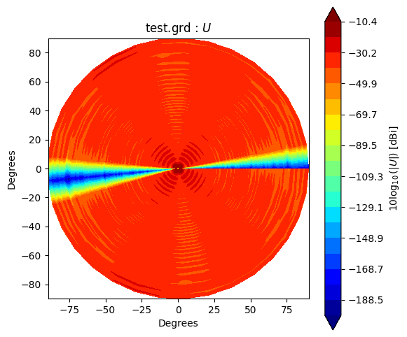
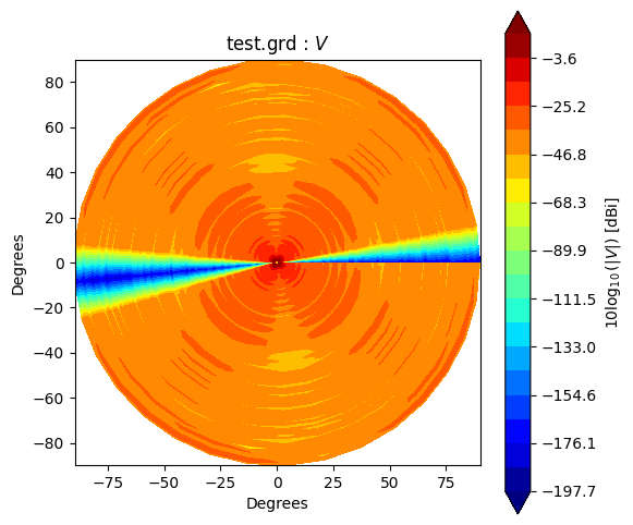
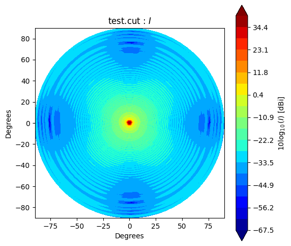
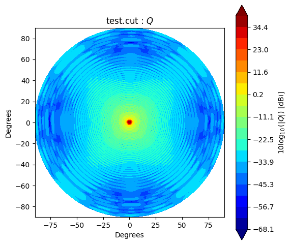
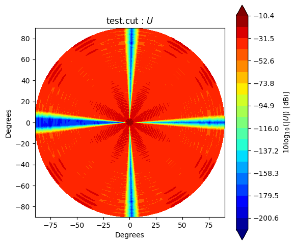
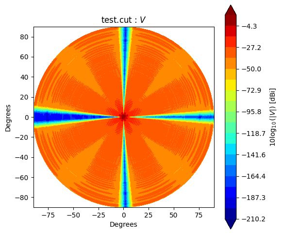
Beam* class has method to_polar which converts grid/cut to Stoke parameter beams.

The instance after conversion has BeamPolar object.

It has the method to plot a Stokes beam as well.

Note that \(Q\) and \(U\) components will be projected after taking an absolute to avoid that \(log()\) has negative value.

g2polar = grid.to_polar(copol_axis="x")
cpolar = cut.to_polar(copol_axis="x")
stokes = ["I", "Q", "U", "V"]
for s in stokes:
    g2polar.plot(s)
for s in stokes:
    cpolar.plot(s)

If you would like to make and accsess the beam plot, you can add return_fields=True to every plot() method. It returns x, y and z values to make a plot.

pol = "co"
x,y,z = cut.plot(pol=pol, return_fields=True)
figsize = 6
plt.figure(figsize=(figsize,figsize))
plt.axes().set_aspect("equal")
plt.title(f"{cut.filename} : {pol}")
plt.xlabel("Degrees")
plt.ylabel("Degrees")
plt.contourf(x, y, 10*np.log10(z), levels=50, cmap='jet', extend='both')
plt.colorbar(orientation="vertical", label="dBi");

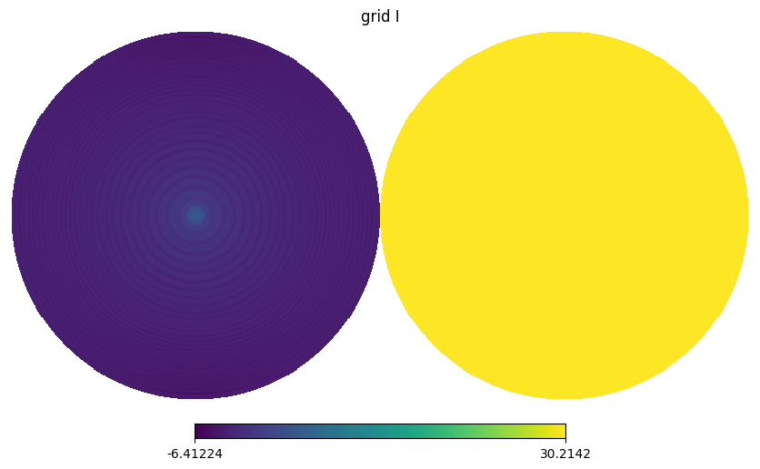
BeamPolar has a method to_map which converts a Stokes beam to HEALPix beam map with specified nside as an argument.

After its operation, new object BeamMap will be generated as an instance.

The beam area that doesn’t have values depending on the GRASP simulation, especially a backside of feed is not often simulated.

By setting outOftheta_val, we can control the value in sky pixel where is not covered by GRASP.

For the converting the BeamPolar to BeamMap, BeamPolar.to_map uses scipy.interpolate.RegularGridInterpolator which has ‘linear’, ‘nearest’, ‘slinear’, ‘cubic’, ‘quintic’ and ‘pchip’ as methods.

nside = 256
outOftheta_val = hp.UNSEEN # Default
gmap = g2polar.to_map(nside, outOftheta_val=outOftheta_val, interp_method="linear")
cmap = cpolar.to_map(nside, outOftheta_val=outOftheta_val)
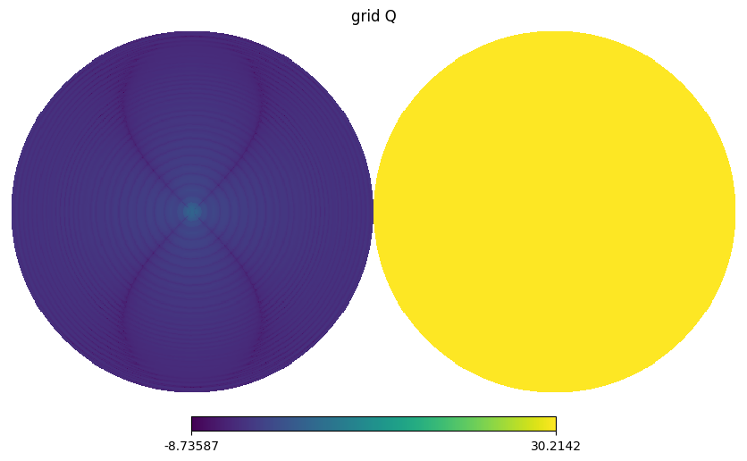
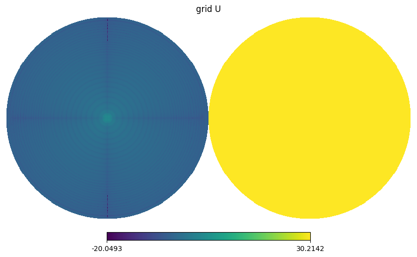
for i,s in enumerate(stokes[:3]):
    hp.orthview(np.log10(np.abs(gmap.map[i])), title=f"grid {s}", rot=(0,90))
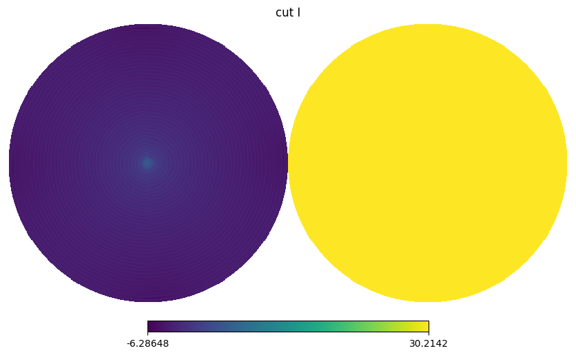
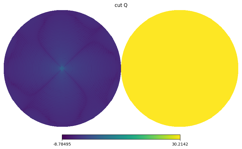
for i,s in enumerate(stokes[:2]):
    hp.orthview(np.log10(np.abs(cmap.map[i])), title=f"cut {s}", rot=(0,90))

BeamMap has a method to_alm which expands a beam map to spherical harmonics coefficients i.e. \(b_{lm}\) with specified lmax and mmax.

galm = gmap.to_alm()
calm = cmap.to_alm()

There is a function grasp2alm that includes every operation which is needed to obtain alm from the GRASP grid or cut file.

galm_ = g2a.grasp2alm(gridfile, nside, interp_method="linear")
calm_ = g2a.grasp2alm(cutfile, nside)

lmax = 3*nside-1
mmax = lmax
galm_lsq = gmap.to_alm_lsq(lmax, mmax)
calm_lsq = cmap.to_alm_lsq(lmax, mmax)
galm_lsq_ = g2a.grasp2alm_lsq(gridfile, nside, lmax, mmax, interp_method="linear")
calm_lsq_ = g2a.grasp2alm_lsq(cutfile, nside, lmax, mmax)